Analysis of Variance
Introduction
Analysis of variance (ANOVA) is a statistical tool that is used to compare variances among different groups.
Parameters
N-Way ANOVA: Whether to perform One-Way ANOVA or Two-Way ANOVA (using either one or two independent variables, respectively).
Outcome: The variable corresponding to the outcome, typically the dependent variable (the variable that is affected by the behavior of independent variables).
Treatment(s): Categorical variable(s) affecting the outcome (the independent variables).
Filters (optional): Set conditions on columns (features), in order to remove any samples in the original dataset which are not required. If selected, only a subset of the original data is used in the analytics.
Case Study 1: Tumors (One-way ANOVA)
Note
This example is available in the Actable AI web app and may be viewed here.
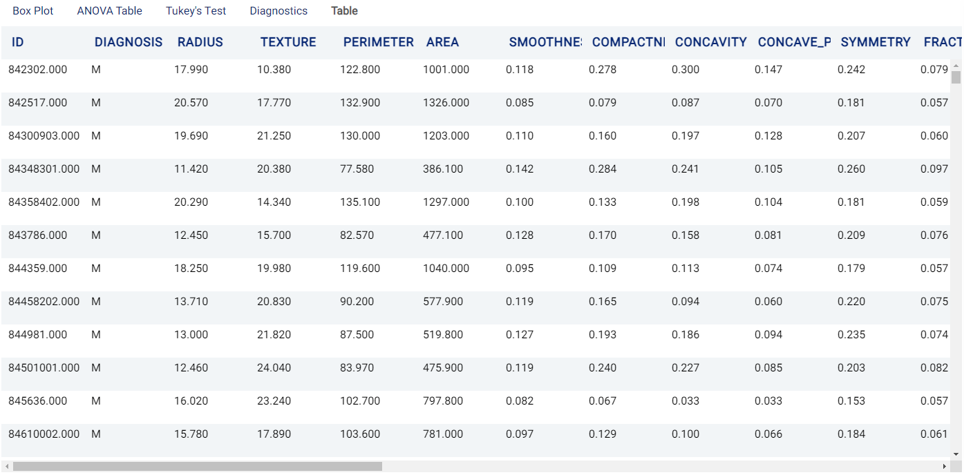
Suppose we are working on tumors and would like to know if a tumor is benign or malignant. A sample of the dataset is as follows:
ID |
Diagnosis |
radius |
texture |
perimeter |
842302 |
M |
17.99 |
10.38 |
122.8 |
842517 |
M |
20.57 |
17.77 |
132.9 |
84300903 |
M |
19.69 |
21.25 |
130.0 |
8510426 |
B |
13.54 |
14.36 |
87.46 |
8510653 |
B |
13.08 |
15.71 |
85.63 |
8510824 |
B |
9.504 |
12.44 |
60.34 |
In this dataset, M represents malignant and B represents benign.
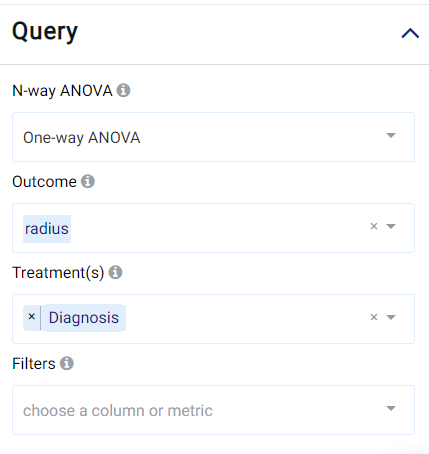
If we would like to have an analysis of variance of the tumor radius (radius) compared with the different diagnosis groups (Diagnosis), the parameters can be set as follows:
The result view contains the Box Plot, ANOVA Table, Tukey’s Test, Diagnostics, and Table tabs:
Boxplot
The distribution of the outcome (radius) grouped by the treatment variable (diagnosis), namely M (malignant) or B (benign), is shown in a box plot. Hovering the mouse cursor over the box plots also reveals further details.
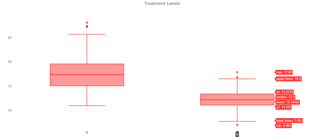
In this image, it is quite clear that malignant tumors have larger radii and greater variations than benign tumors.
ANOVA Table
The ANOVA Table tab shows the results of the ANOVA analysis, an example of which is shown in the following image:
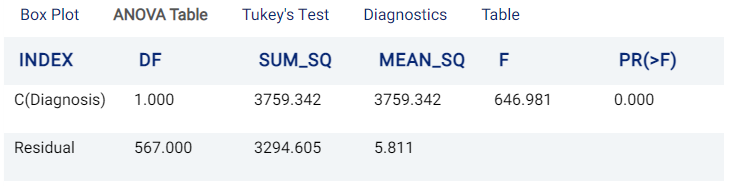
In the table, DF stands for Degrees Of Freedom, SUM_SQ refers to Sum of Squares, MEAN_SQ refers to Mean Squares, F refers to the F test statistic (the mean square of the variable divided by the mean square of each parameter), and PR(>F) refers to the probability (P-Value) of the F value being greater than the observed value. The Null Hypothesis (which states that any differences are not statistically significant and have occurred only due to chance) is rejected if this probability is less than or equal to a significance level known as the alpha value. More information can be viewed here.
In this example, the PR(>F) value of 0 indicates that there is a statistically significant difference in the effect between different classes of Diagnosis on radius.
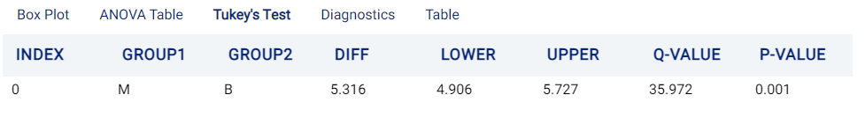
Tukey’s Test
The Tukey’s Test tab shows the results of the Tukey’s range test analysis. More information on this test can be viewed here.
Diagnostics
The Diagnostics tab is composed of several sub-tabs, as follows:
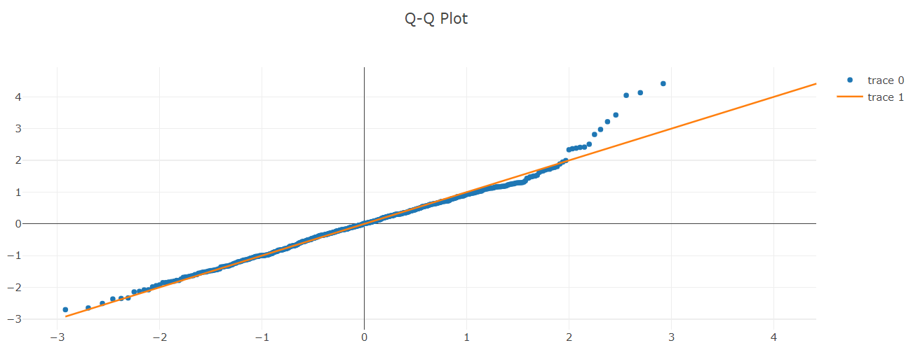
Q-Q Plot
This tab shows the quantile-quantile plot (Q-Q plot) of the ANOVA analysis. The Q-Q plot is a graphical representation of two probability distributions by comparing their quantiles. The \(x\)-axis represents the quantiles for the normal distribution and the \(y\)-axis contains the quantiles of the data. Hence, the Q-Q Plot indicates if the data is similar to the normal distribution.
Distributions which are similar to each other will lie approximately on the identity line ( \(y\) = \(x\) ) labeled ‘trace 1’ (orange line) in the graph. On the other hand, distributions which are linearly related will also lie on a line but not necessarily on the identity line.
More information on the Q-Q plot is available here.
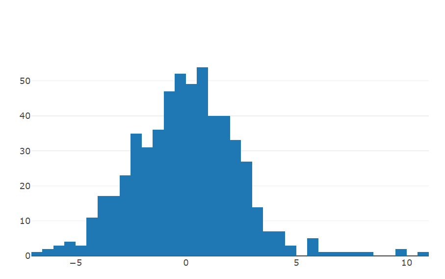
Residual Plot
The Residual Plot tab shows the residuals of the ANOVA analysis. Residuals correspond to differences between the data and the fitted values. If the residuals are not randomly distributed, then a linear regression model is suitable for the data.
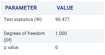
Shapiro Wilk
This tab shows the results of the Shapiro-Wilk test, which is a non-parametric test for normality. Specifically, the Shapiro-Wilk test is used to determine whether to accept or reject the Null Hypothesis that the data is normally distributed. If the P-Value is less than the chosen alpha value, the Null Hypothesis is rejected and it can thus be deduced that the data is not normally distributed.
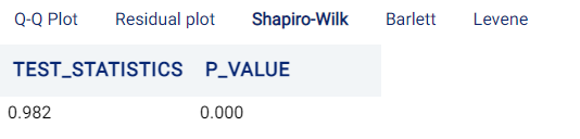
More information on the Shapiro-Wilk test can be viewed here.
Bartlett
This tab shows the results of Bartlett’s test, used to test homoscedasticity (i.e. testing if variances are equal across groups or samples, an assumption made by some statistics tests such as ANOVA). If the p-value is less than the alpha value, the Null Hypothesis (postulating that there is no difference in variances) is rejected, concluding that there are differences between variances that are unlikely to have occurred by chance.
More information can be viewed here.
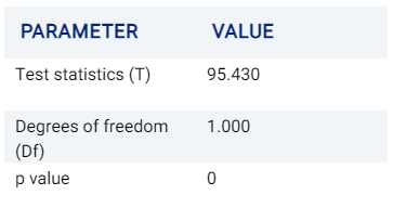
It is known that Bartlett’s test is sensitive to departures from normality (i.e. cases where samples are derived from non-normal distributions). Levene’s test is an alternative test that is less sensitive to such departures from normality.
Levene
Levene’s test is similar to Bartlett’s test described above in testing for equality of variances across multiple samples or groups, but is less sensitive to departures from normality.
More information on Levene’s test can be viewed here.
Case Study 2: Apartment Rental Prices (Two-way ANOVA)
Note
This example is available in the Actable AI web app and may be viewed here.
Suppose we are a real estate agent and we would like to predict the rental price for different apartments based on features such as their size, location, etc. A sample of a dataset containing this information is as follows:
number_of_rooms |
number_of_bathrooms |
sqft |
location |
days_on_market |
initial_price |
neighborhood |
rental_price |
|---|---|---|---|---|---|---|---|
0 |
1 |
484,8 |
great |
10 |
2271 |
south_side |
2271 |
1 |
1 |
674 |
good |
1 |
2167 |
downtown |
2167 |
1 |
1 |
554 |
poor |
19 |
1883 |
westbrae |
1883 |
0 |
1 |
529 |
great |
3 |
2431 |
south_side |
2431 |
3 |
2 |
1219 |
great |
3 |
5510 |
south_side |
5510 |
1 |
1 |
398 |
great |
11 |
2272 |
south_side |
2272 |
3 |
2 |
1190 |
poor |
58 |
4463 |
westbrae |
4123.812 |
If we would like to analyze how the variance of the rental price behaves across different types of locations and across a varying number of rooms, 2-way ANOVA could be employed with the following parameters:
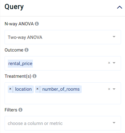
The result view is similar to the first case study (so that it again contains the Box Plot, ANOVA Table, Tukey’s Test, Diagnostics, and Table tabs), but now considers the variance of two treatment variables with the outcome:
Boxplot
The distribution of the outcome (rental_price) grouped by both treatment variables (location and number_of_rooms) is shown in a box plot. Hovering the mouse cursor over the box plots also reveals further details.
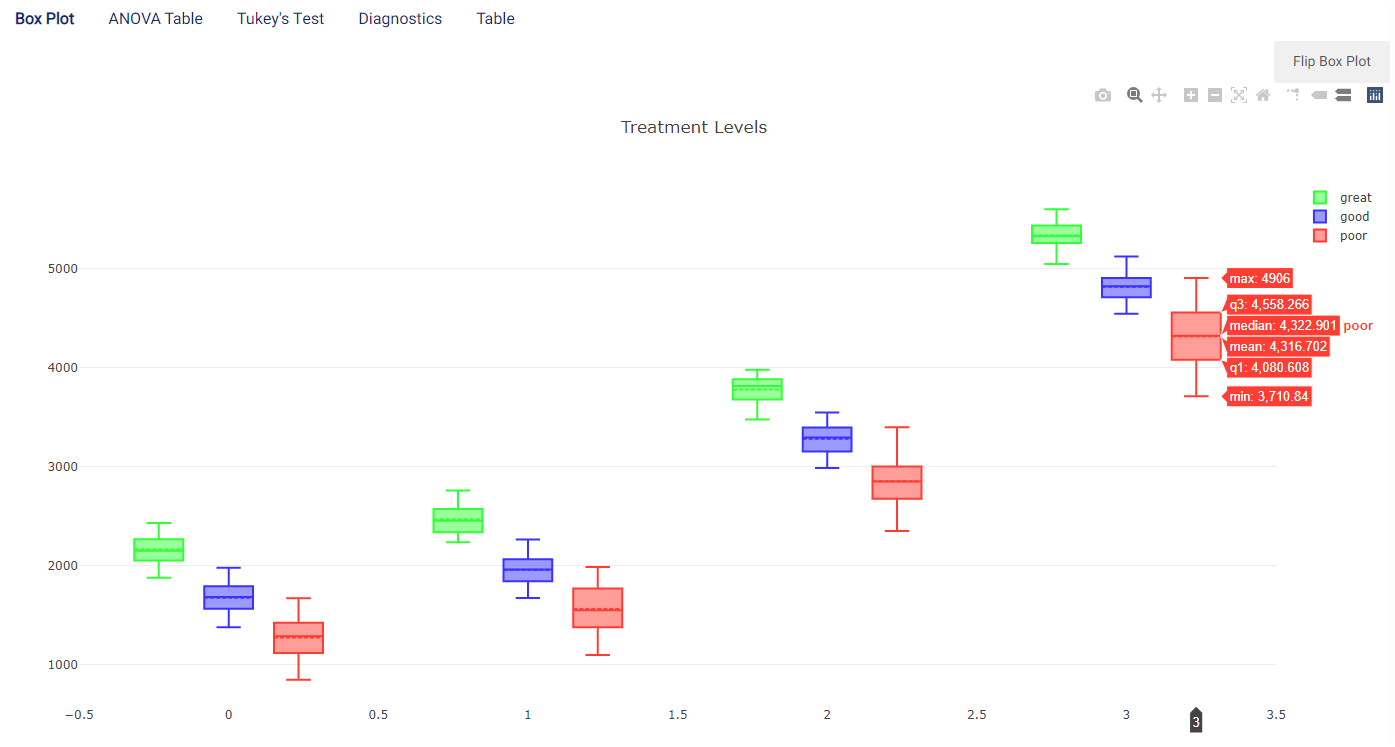
In this image, the \(x\)-axis represents the location while there is then one box plot for each value of number_of_rooms present in the dataset (i.e. between 0 and 3 rooms).
The box plot can be flipped by clicking on the Flip Box Plot button, to represent the number_of_rooms on the \(x\)-axis with each value containing one box plot for each location:
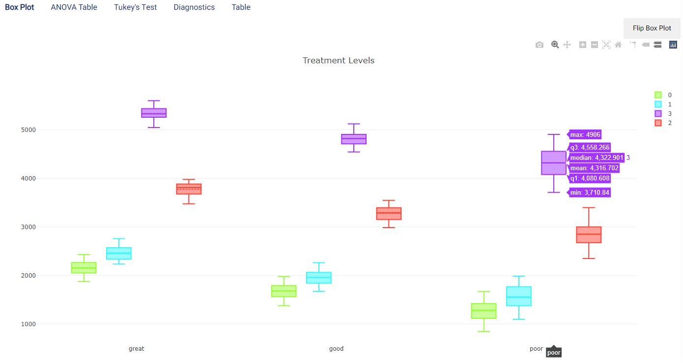
It is clear from both box plots that the rental price increases as the number of rooms increases, and poor locations are generally worth less rent than good locations which are in turn worth less than great locations. However, it can also be observed that there are large variances for poor properties, so that some of these may have a similar rental price to good properties.
Two-way ANOVA can be helpful to separate the effects of the two treatment variables. For example, if One-way ANOVA is performed using location as the treatment, the following is obtained:
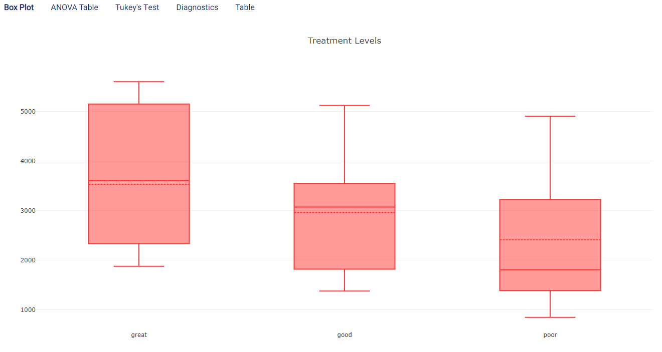
As can be observed, while there is again a general trend that poor apartments are worth less than good apartments which are in turn worth less than great apartments, it is much less clear than before. This is due to the substantial variances and overlaps between groups. The inclusion of the number of rooms thus enabled better separation and understanding of how the rental price varies across both treatment variables.
ANOVA Table
The ANOVA Table tab shows the results of the ANOVA analysis, using both treatment variables. An example of which is shown in the following image:
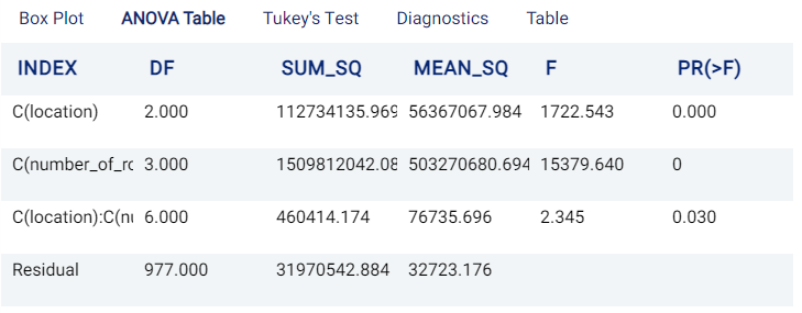
The interpretation of the table is similar to the One-way ANOVA case: ANOVA Table. In this example, both the location and number_of_rooms have statistically significant effects on the rental_price.
Tukey’s Test
The Tukey’s Test tab shows the results of the Tukey’s range test analysis. More information on this test can be viewed here.
In the case of Two-way ANOVA, there is one tab for each treatment, containing a table with one row for each pair of possible groups. For example, in the case of location spanning values poor, good, and great, the following (order-invariant) pairs are possible:
Poor, Good
Poor, Great
Good, Great
This results in three rows (one for each pair), while there are six rows in the case of number_of_rooms:
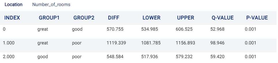
Tukey’s Test for location (and rental_price)
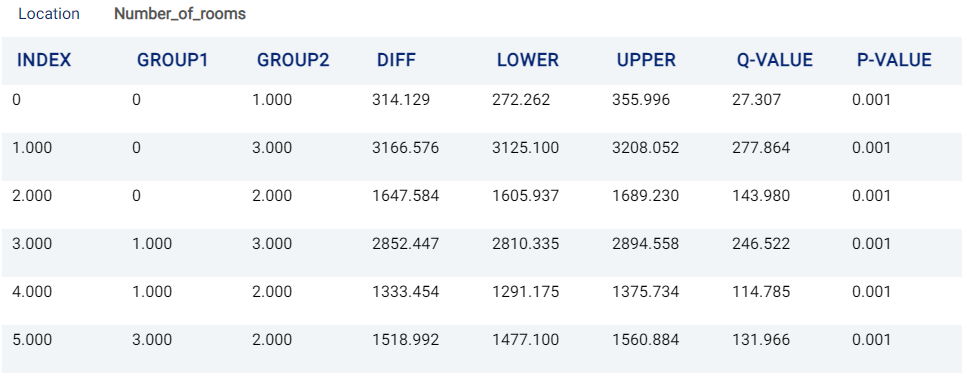
Tukey’s Test for number_of_rooms (and rental_price)
From the two tables above, it is evident that there are statistically significant differences between all groups in this example.
Diagnostics
The Diagnostics tab is composed of several sub-tabs that are largely identical to the One-way ANOVA case. See Diagnostics for more information.