Counterfactual Analysis
Introduction
Counterfactual Analysis helps to predict outcomes when one of the inputs is changed. For example, it can help predict customer demands if prices change, or predict disease outcome if a treatment is taken. This is different from ‘What-if’ analysis of predictive models that generates results by predicting outcomes from a new input value.
To understand the difference between our counterfactual analysis and ‘What-if’ analysis, it is important to understand the difference between an intervention and an observed value: an intervention is an action taken that changes one of the input values, while an observed value is simply what is observed and we do not know the source or cause of the change. To predict the outcome of an intervention, it is essential to estimate the causal effect of the intervention on the outcome. Hence, counterfactual analysis provides an understanding of how an outcome is affected by changes to input values via an intervention, and similarly, what changes to the input values would change a model’s outcomes and decisions.
In order to avoid biases due to spurious correlations, common causes (also known as confounders, which affect both the treatment and outcome variables) are first disassociated from both the given treatment variables and the outcome variable. It then finds the association between the disassociated treatment and outcome variables. This process is done using Double Machine Learning, which first generates two predictive models (to predict the outcome from the confounder variables, and to predict the treatment from the confounders), that are then combined to create a model of the treatment effects.
To run a Counterfactual Analysis, the following are required:
A dataset that contains the outcome
The values of the treatment variable
The new values of the treatment variable
The common causes that have causal effects on both the treatment and outcome
Parameters
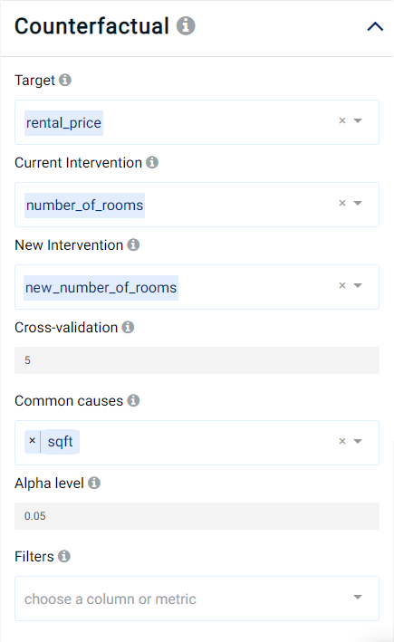
Target: The variable on which we want to measure the effects of the intervention, a.k.a. the outcome. It can only be numerical.
Current Intervention: Variables that cause the effect of interest, a.k.a. the current treatment affecting the outcome. It can be either numeric, Boolean, or categorical.
New Intervention: New variable that will generate a different effect on the outcome, a.k.a. the new treatment affecting the outcome. It can be either numeric, Boolean, or categorical. It must be the same type as the Current Intervention.
Cross-validation: Number of folds to use in cross-validation for the double machine learning algorithm. A larger value leads to better results but makes the analysis slower. Default value is 5.
Common causes: Also known as confounders, these are variables that can affect both the treatment and the outcome. Selecting good common causes can help improve the results. The columns that have an effect on both the target and the current intervention should be included.
Alpha level: Value used to calculate the lower and upper bounds of the effect. For example, if the alpha effect is 0.05, the lower bound and upper bound would create a 95% confidence interval for the effect. Default is 0.05.
Filters (optional): Set conditions on the columns to be filtered in the original dataset. If selected, only a subset of the original data will be used in the analytics.
Furthermore, if any features are related to time, they can also be used for visualization:
Time Column: The time-based feature to be used for visualization. An arbitrary expression which returns a DATETIME column in the table can also be defined, using format codes as defined here.
Time Range: The time range used for visualization, where the time is based on the Time Column. A number of pre-set values are provided, such as Last day, Last week, Last month, etc. Custom time ranges can also be provided. In any case, all relative times are evaluated on the server using the server’s local time, and all tooltips and placeholder times are expressed in UTC. If either of the start time and/or end time is specified, the time-zone can also be set using the ISO 8601 format.
Result View
Table: A table showing the counterfactual effect of the treatment on the outcome. The columns are the same as the original data set but new columns are added to show the counterfactual effect:
The
<target>_intervenedcolumn shows the outcome after the intervention, where <target> represents the name of the Target variable.The
<target>_intervened_highand<target>_intervened_lowcolumns show the upper and lower bounds, respectively, of the counterfactual effect.The
intervention_effectcolumn shows the difference between the intervened outcome and the original outcome.The
intervention_effect_highandintervention_effect_lowcolumns show the difference between the intervened outcome and the original outcome’s upper and lower bounds, respectively, of the counterfactual effect.
Validation: Shows the validation results of the double machine learning algorithm:
The treatment model infers the treatment from the common causes.
The outcome model infers the outcome from the common causes.
A final model is then used on the residuals of the treatment and outcome models to infer the counterfactual effect.
The Feature-Importance tables show the importance of each variable in the models.
The residual plot shows the residuals of the outcome model on the \(y\)-axis, and the residuals of the treatment model on the \(x\)-axis.
Causal graph: A Directed Acyclic Graph (DAG) that visualizes the parameter choices based on user selection of treatment, outcome and common causes. A DAG (an example of which is shown below) can be interpreted as follows:
An edge represents causality between variables.
Gray color represents the Common causes variables.
White color represents the Current Intervention variable.
Red color represents the Outcome variable.
Plot:
The first graph depicts the intervention chart, namely a plot of the original target on the \(x\)-axis, and the intervened target on the \(y\)-axis. If the target increases, the point will be above the identity line (the line on which the original target and new intervened target are equal). If the target decreases, the point will be below the identity line. If the intervention is categorical, the points will have colors corresponding to each pair of categories (
current_intervention->new_intervention). If the intervention is numeric, the point will have a color corresponding to the value of the difference of the interventions (new_intervention-current_intervention).The second plot is the effect plot; if numerical, the \(x\)-axis is the difference of the interventions, whereas if categorical, the \(x\)-axis contains each pair of categories. The \(y\)-axis is the intervention effect (
new_target-original_target).
Case Study
Note
This example is available in the Actable AI web app and may be viewed here.
Suppose that we are a real estate agent and we would like to see how the price of a house changes if the number of rooms is increased or decreased.
To do this, we use an existing dataset of houses and add a new column called new_number_of_rooms representing the number of rooms after the intervention, where our intervention is number_of_rooms + random.choice([-1, 1]) (i.e. the number of rooms is randomly increased or decreased by 1).
An example of the dataset is as follows:
number_of_rooms |
new_number_of_rooms |
sqft |
rental_price |
|---|---|---|---|
0 |
1 |
484.8 |
2271 |
1 |
2 |
674 |
2167 |
1 |
0 |
554 |
1883 |
0 |
1 |
529 |
2431 |
3 |
2 |
1219 |
5510 |
1 |
2 |
398 |
2272 |
3 |
2 |
1190 |
4123.812 |
To run the counterfactual analysis, we need to specify the following parameters:
The target is the column
rental_price.The current intervention is the
number_of_rooms.The new intervention is the column
new_number_of_rooms.The common cause is the column
sqft.
After pressing the Run button, the following will be displayed:
Table
A table containing the counterfactual effect of the treatment on the outcome for each appartment.
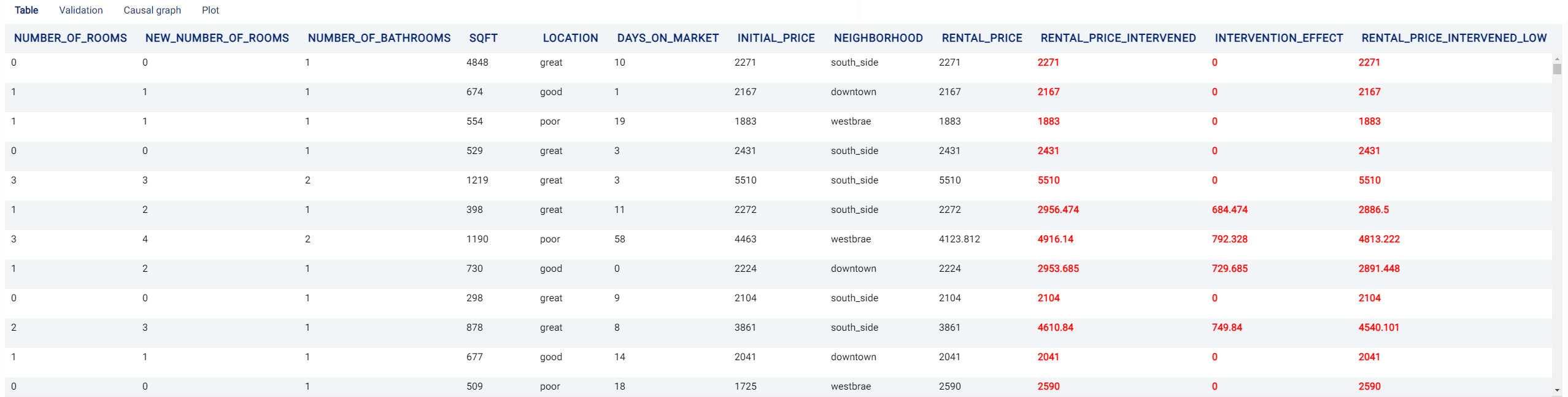
This table can be downloaded by clicking on the Download button.

Validation
This tab shows the validation results for the double machine learning models:
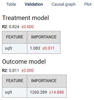
It can be observed that the treatment model and the outcome model have been able to infer the common causes, meaning that the rental price and the number of rooms can be easily found with the sqft feature alone.
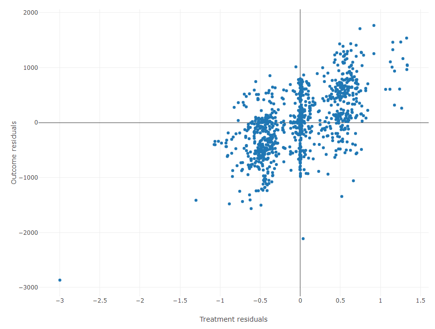
In the above image, the residuals of the two models can be observed.
Causal Graph
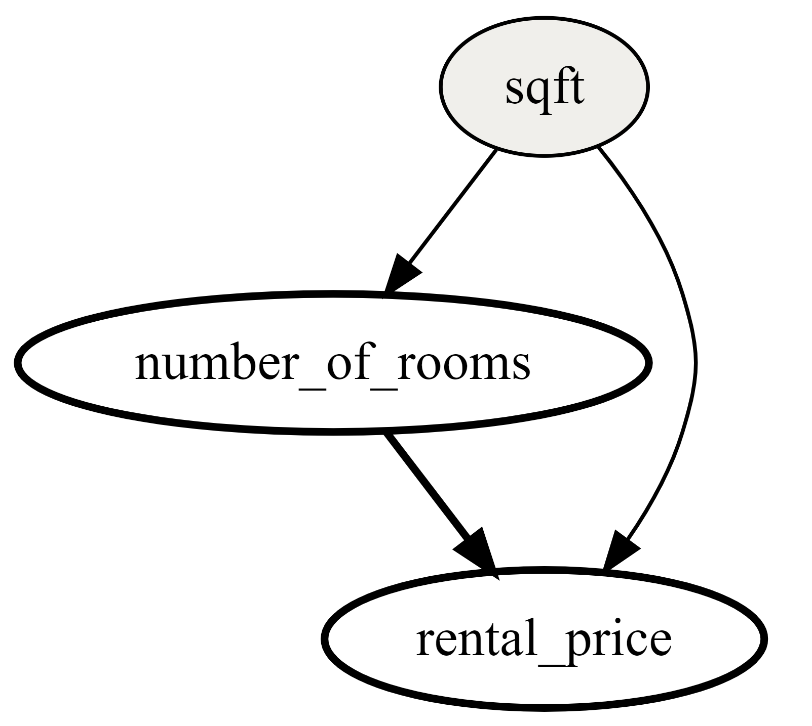
The causal graph helps to visualize the causal relationships between the variables. From the graph, we can see that sqft is a cause of the rental_price and number_of_rooms, and that number_of_rooms is also a cause of the rental_price.
Intervention Plot
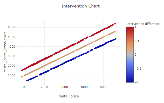
The \(x\)-axis represents the original rental price, while the \(y\)-axis represents the predicted rental price after the intervention. The color of each point corresponds to the difference in the number of rooms: a red point indicates that the number of rooms was incremented by 1, while a blue point indicates that the number of rooms was decreased by 1.
It can be observed that the rental price is generally higher when the number of rooms increases, as could be expected.
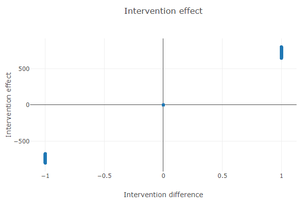
In this plot, we can see the range of the effect of the intervention. The \(x\)-axis contains the intervention difference (new_number_of_rooms - number_of_rooms) and the \(y\)-axis represents the effect of the intervention (rental_price - rental_price_intervened). It can also be observed from this plot that decreasing the number of rooms always results in a decrease in the price, whereas increasing the number of rooms generally results in a higher price.