Debias
Introduction
Some features in a dataset might be biased and may affect the prediction of the desired values and may also affect other features in the dataset. Hence, it is not sufficient to exclude such a feature from being used in training, because it might still be reflected in other features.
In these cases, Actable AI offers the possibility to debias features from datasets to enable unbiased predictions. By extrapolating the debiased features with the biased groups, Actable AI’s algorithm calculates residual values of this prediction and uses them to obtain unbiased results. This process attempts to remove the impact of the biased feature on the final prediction by removing its impact on the other features.
Parameters
Sensitive Groups: Groups that are biased and are creating bias in other features of the dataset.
Proxy Features: Features that are correlated with the Sensitive Groups and need to be debiased.
Evaluation
Actable AI’s debias feature works for both Classification and Regression. The debias feature is demonstrated using the following biased datasets:
Classification: Data on passengers travelling on the Titanic.
Regression: Glassdoor base pay records.
Classification
One of the most famous maritime disasters is the sinking of the RMS Titanic on 15 April 1912. There is post-disaster research indicating that passengers’ survival chances depended on the class in which they were travelling, with people travelling in first class having higher chances to survive.
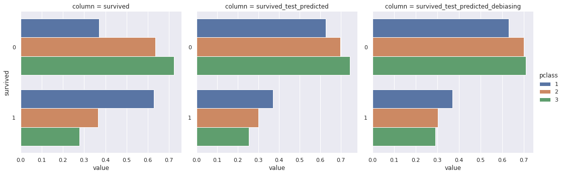
We manually select a subset of data as our prediction dataset which ensures that our prediction dataset has an equal distribution of survivors for different travelling classes. However, the prediction result indeed shows that there are not equal chances of survival for different passenger classes.
By enabling Actable AI’s debias feature, we can observe a significant improvement in the distribution, thereby demomnstrating the effectiveness of the algorithm for other cases that could benefit from debiasing when performing classification. The following image shows (from left to right): (1) the survival distribution across first, second and third-class passengers for the original dataset, (2) prediction without debias, and (3) prediction with debias enabled. The $x$-axis shows the possibility of survival, and the $y$-axis values represent ‘survived’ (1) and ‘not survived’ (0).
Regression
As we may know, the gender pay gap is a real-world discrimination problem that shows a difference between the remuneration among different genders. We will use the Glassdoor dataset that indicates the distribution for the base pay across males and females to illustrate this problem.
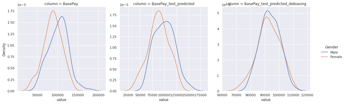
Due to the nature of the data distribution in this dataset, the prediction result is also biased, even after manually selecting the prediction dataset to have the same base pay distribution for males and females. The prediction result for base pay shows a clear bias that females are underpaid compared to males, and the distribution is inclined to align with the original dataset.
By enabling our debias feature, we can clearly observe a significant improvement in the distribution, indicating that the bias between genders has been largely mitigated and the model is fairer across genders when estimating the base pay. The following image shows (from left to right): (1) the base pay distribution across males and females for the original dataset, (2) prediction without debias, and (3) prediction with debias enabled. The x-axis represents the base pay value, and y-axis represents the density.
Performance Impact
Enabling the debias functionality might slightly impact your model’s performance.
In the Titanic example, the prediction accuracy dropped from 76.033% (for the model trained without debias) to 69.421% (for the model trained using debias), representing a 6.6% drop in performance. The Area Under Curve (AUC) score also decreased from 0.775 to 0.759 (a drop of 0.016).
For the base pay prediction example, the debiased model attained a Root Mean Squared Error (RMSE) of 24,595.627, whereas the model without debias attained a lower Root Mean Squared Error (RMSE) value of 10,819.215.