Bayesian Linear Regression

Introduction

Similarly to Regression, Bayesian Linear Regression analysis predicts a continuous value based on other variables, and also provides data which helps to interpret the results.

Actable AI uses the entire table as the source data and automatically splits the table into three parts:

• Training data: Rows in the table where both the predictors and the ground-truth target are known and available. More information available here.

• Prediction data: Rows where target column is missing, and thus need to be predicted.

• Validation data: Actable AI samples a part of the data to verify the reliability of the trained model. This part of the data is also used in the performance tuning stage if performance optimization is selected. More information available here.

Parameters

There are two tabs containing options that can be set: the Data tab, and the Priors tab, as follows:

• Data tab:

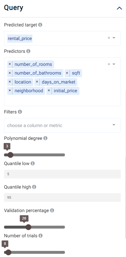
  • Predicted target: Choose one column for which any missing values should be predicted.

  • Predictors: Columns that are used to predict the predicted target.

  • Validation percentage: The model is trained with the training set and is validated (tested whilst performing training) using the validation set. By sliding this value, one can control the percentage of rows with a non-empty predicted target that is used for validation.

  • Polynomial degree: Calculate exponential and cross-intersection values for numeric variables, the values would be used as additional input.

  • Quantile low: Used to calculate the lower bound of the prediction interval. More information available here.

  • Quantile high: Used to calculate the upper bound of the prediction interval. More information available here.

  • Filters (optional): Set conditions on columns (features), in order to remove any samples in the original dataset which are not required. If selected, only a subset of the original data is used in the analytics.

  • Number of trials: Number of trials for hyper-parameter optimization. Increasing the number of trails usually results in better prediction but longer training time.

  Furthermore, if any features are related to time, they can also be used for visualization:

  • Time Column: The time-based feature to be used for visualization. An arbitrary expression which returns a DATETIME column in the table can also be defined, using format codes as defined here.

  • Time Range: The time range used for visualization, where the time is based on the Time Column. A number of pre-set values are provided, such as Last day, Last week, Last month, etc. Custom time ranges can also be provided. In any case, all relative times are evaluated on the server using the server’s local time, and all tooltips and placeholder times are expressed in UTC. If either of the start time and/or end time is specified, the time-zone can also be set using the ISO 8601 format.

• Priors:

  Optionally, the priors can be set. The prior of a certain quantity is the probability distribution that reflects one’s beliefs about the likely values of this quantity before any data is seen or taken into account.

  By clicking on the green Add Prior button, a new prior can be added:

  

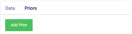
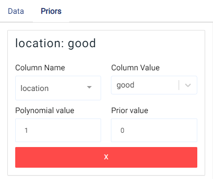
  The following fields then need to be filled:

  • Column Name: the name of the column to be used as a prior. If the type of the column is double, then the Prior value can be set. Otherwise, the Column value should be set.

    Note

    Fields which cannot be set are grayed out to avoid mistakenly filling in any incorrect values.

  • Column Value: The value of the column variable to be used (can only be set if the Column Name type is not of type double).

  • Polynomial value: Maximum polynomial degree to be used. Highest value that can be used is 3.

  • Prior value: The value of the prior to be used.

  

Case Study

Note

This example is available in the Actable AI web app and may be viewed here.

Suppose we are working at a real estate company and would like to forecast rental prices for properties that remain on the market. The below table represents a sample of the dataset:

days_on_market	initial_price	location	neighborhood	number_of_bathrooms	number_of_rooms	sqft	rental_price
10	2271	great	south_side	1	0	4848	2271
1	2167	good	downtown	1	1	674	2167
19	1883	poor	westbrae	1	1	554	1883
3	2431	great	south_side	1	0	529	2431
58	4463	poor	westbrae	2	3	1190	4123.812

Now, we have added some new properties and would like to find out the rental price given their condition:

days_on_market	initial_price	location	neighborhood	number_of_bathrooms	number_of_rooms	sqft	rental_price
18	1725	poor	westbrae	1	0	509
49	1388	poor	westbrae	1	0	481
1	4677	good	downtown	2	3	808
30	1713	poor	westbrae	1	1	522
10	1903	good	downtown	1	1	533

We set our parameters as follows:

Review Result

The result view contains a Prediction tab, a Performance tab, a Multivariate tab, a Univariate tab and a Table tab.

Prediction

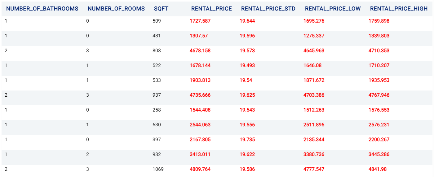
The Prediction tab shows the prediction result for the rows where the target value was missing. The table has several new columns, where <target> is the name of the target variable:

• <target>: the predicted values of the target variable.

• <target_STD>: the standard deviation of predicted values.

• <target>_low and <target>_high: these columns represent the lower and upper quartile bounds, respectively, of the predicted price given the values set for Quantile low and Quantile high, respectively.

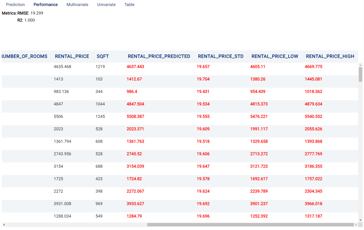
Performance

The Performance tab shows the performance of the model with the Root Mean Square Error (RMSE) metric (19.299) and the R-squared (R2) metric (1.0).

• Root Mean Square Error (RMSE): Calculated as the square root of the second sample moment of the differences between the predicted and observed values.

• R-squared (R2): Also known as the coefficient of determination, and indicates the extent to which a target variable is predictable from the predictor variables. A value of 0 means that predictors have zero predictability of the target, while a value of 1 means the target is fully predictable by the predictors.

Multivariate

The Multivariate tab contains a table showing information related to the behavior of the predictions when multiple variables are considered.

• Variable name: The name(s) of the variable(s) used. Multiple variable names correspond to a cross-intersection of variables. In simple terms, these variables are essentially multiplied by each other.

• Coefficient Value: Coefficients of the regression model (mean of the distribution), which can give an indication as to the variables’ importance. Values close to 0 are unimportant and largely unused when predicting the target. Larger values (even if they are negative) indicate that the variable(s) highly influence(s) the predictions.

• Standard Deviation: Standard deviation values of the coefficients.

Univariate

The information in this tab focuses more on the relationship between the target and each individual predictor. A univariate analysis is generated for every original value (every non cross-intersection or exponent) in the dataset. For example, in the case of categorical values such as location which can take values of great, good, and poor, analyses using each of these values is provided (i.e. location_great, location_good, and location_poor).

Two graphs are generated for each variable considered:

• The first graph shows a regression of our target (rental price in our example) by only using the number of rooms as a feature that can be used for prediction. An example is shown in the image below. It can be observed that the number of rooms can easily predict the rental price with an R-squared value of 0.912. It can also be observed that the price increases when the number of rooms increases.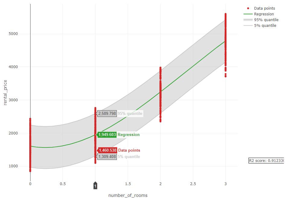

  

• The second graph shows the Probability Density Function (PDF) of the target (rental price). It is also evident in this graph that the number of rooms has a positive influence on the price.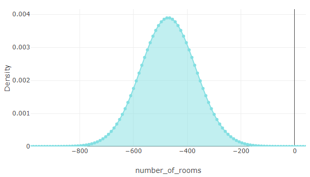

  

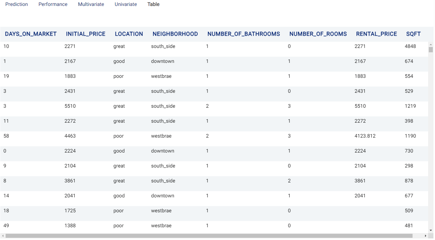
Table

The Table tab displays the first 1,000 rows in the original dataset and the corresponding values of the columns used in the analysis: