Correlation Analysis
Introduction
Correlation analysis is a method of statistical evaluation used to study the relationship between two variables. This analysis is useful to indicate whether there are any connections between variables in the same dataset, and what is the magnitude and effect of that relationship.
As an example, in the advertising industry, there is normally a correlation between advertising spend and the advertisements’ impression rate, such that a higher advertising spend tends to result in higher impression rates.
It should be noted that correlation is not always causal, with most relationships tending to be misleading and showing fake relationships between variables. In order to discover and understand the true causal, you may use Actable AI’s Causal Inference analytic.
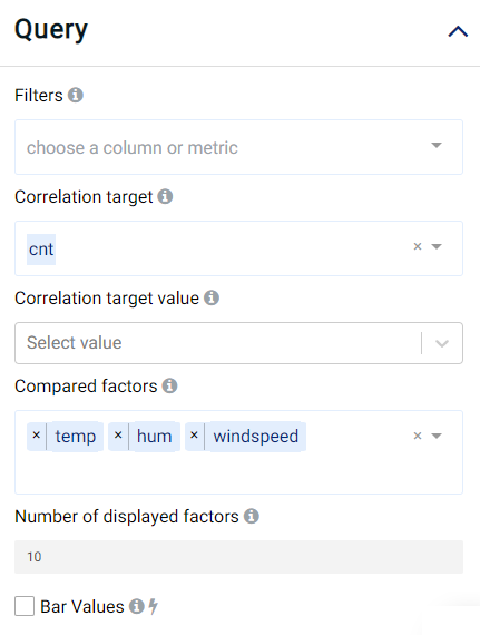
Parameters
Compared factors: Features for which their correlation with the target will be computed.
Correlation target: The feature to be studied with selected Compared factors.
Number of displayed factors: Number of best-correlated factors to be displayed.
Correlation target value (optional): If set, the target is treated as a binary variable. Samples with the chosen value will be set as positive, while the rest of the classes are set to negative.
Filters (optional): Set conditions on columns (features) so as to remove any samples in the original dataset which are not required. If selected, only a subset of the original data is used.
Bar Values: If selected, values are shown on the bar. Changing this control takes effect instantly in the visualizations.
Furthermore, if any features are related to time, they can also be used for visualization:
Time Column: The time-based feature to be used for visualization. An arbitrary expression which returns a DATETIME column in the table can also be defined, using format codes as defined here.
Time Range: The time range used for visualization, where the time is based on the Time Column. A number of pre-set values are provided, such as Last day, Last week, Last month, etc. Custom time ranges can also be provided. In any case, all relative times are evaluated on the server using the server’s local time, and all tooltips and placeholder times are expressed in UTC. If either of the start time and/or end time is specified, the time-zone can also be set using the ISO 8601 format.
Case Study
Note
This example is available in the Actable AI web app and may be viewed here.
Suppose that we are a bike rental shop owner. We have our bike demand data for the past two years and we would like to understand the effect of the weather change on the bike rental demand. All weather values are normalized in the dataset, an example of which is given below:
temp |
hum |
windspeed |
casual |
registered |
cnt |
dteday |
|---|---|---|---|---|---|---|
0.344167 |
0.805833 |
0.160446 |
331 |
654 |
985 |
2011-01-01 |
0.363478 |
0.696087 |
0.248539 |
131 |
670 |
801 |
2011-01-02 |
0.196364 |
0.437273 |
0.248309 |
120 |
1229 |
1349 |
2011-01-03 |
0.2 |
0.590435 |
0.160296 |
108 |
1454 |
1562 |
2011-01-04 |
0.226957 |
0.436957 |
0.1869 |
82 |
1518 |
1600 |
2011-01-05 |
0.204348 |
0.518261 |
0.0895652 |
88 |
1518 |
1606 |
2011-01-06 |
0.196522 |
0.498696 |
0.168726 |
148 |
1362 |
1510 |
2011-01-07 |
0.165 |
0.535833 |
0.266804 |
68 |
891 |
959 |
2011-01-08 |
0.138333 |
0.434167 |
0.36195 |
54 |
768 |
822 |
2011-01-09 |
We set our parameters as follows, where cnt stands for the rental demand count.
Review Result
The result view contains a Chart tab, a Correlation Result tab and a Data tab:
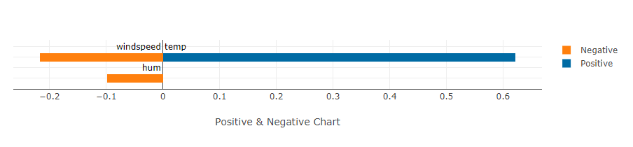
Chart
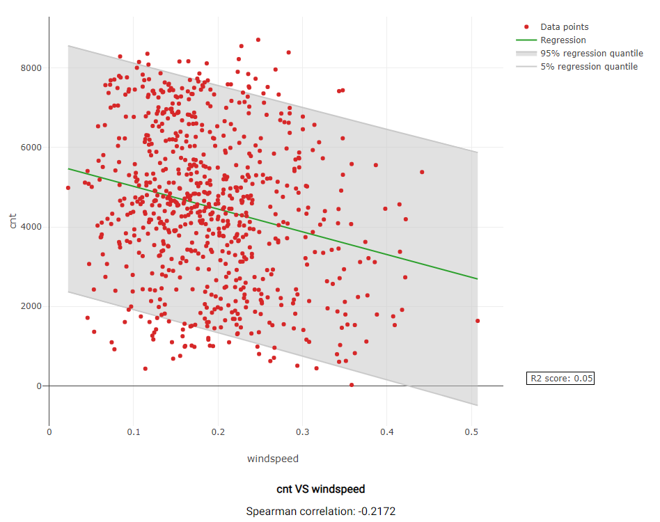
The Chart tab provides an overview plot chart for showing the correlation between Compared factors and Correlation target. As can be observed, temp has a positive correlation with cnt while windspeed and hum (humidity) has negative correlation with cnt.
Actable AI also gives breakdown views for all Compared factors. For example, the following graph describes the correlation between temp and cnt. Most of data points are well-explained by the regression calculation, with a correlation coefficient of 0.622.
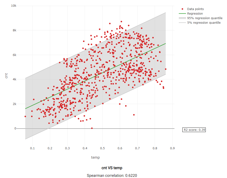
Actable AI uses the Spearman’s Rank-Order Correlation Coefficient (SROCC) to indicate the strength and direction of the correlation. More information on SROCC can be found here.
In the image above, the SROCC has a positive value and it can be clearly observed that cnt tends to increase with increasing values of temp. On the other hand, the image below shows that cnt tends to decrease with increasing values of windspeed, although this relationship is quite weak with a magnitude of 0.2172. These results make sense, since people might feel uncomfortable riding a bike when it is cold or when it is windy.
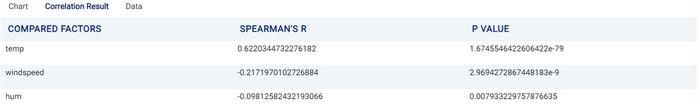
Correlation Result
This tab provides the Spearman’s Rank-Order Correlation Coefficient values and the p-values for the correlation of each factor with the target. The p-value is a measure of how likely any observed correlation is due to chance, with the null hypothesis stating that there is no correlation between a factor and the target. The range of p-values lies between 0 (0%) - 1 (100%):
A value close to 1 indicates that the null hypothesis is true. Hence, there is no correlation between the compared variables.
A value close to 0 suggests that the null hypothesis should be rejected. Hence, there is a high probability that the feature truly does exhibit the observed correlation (and thus the result did not occur by chance).
The threshold at which the null hypothesis is accepted or rejected is known as the alpha value and is typically set to 0.05, meaning that the probability of achieving the same or more extreme results is 5% under the assumption that the null hypothesis is true. The null hypothesis is rejected if the p-value is less than the alpha value.
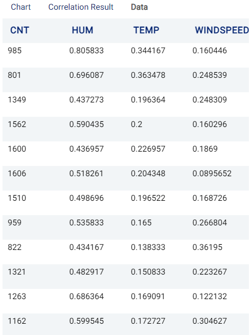
Data
The Data tab displays the first 1,000 rows in the original dataset and the corresponding values of the columns used in the analysis: